What are the steps to find the inverse of a nonsingular 3 x3 matrix?

Introduce unity at the intersection of the first row and the first column either by interchanging two rows or by adding a constant multiple of elements of some other row to the first row. After introducing unity at (1,1) place introduce zeros at all other places in the first column. Introduce unity at the intersection of the 2nd row and 2nd column with the help of the 2nd and 3rd row.

Are row transformation and column Transformation the same?

No, Row transformation and column Transformation are different because, In Elementary row transformation, rows are the only ones that are altered. Whereas In the Elementary column transformation, the matrices' columns are the only ones that are altered.

While performing row operations, is the entire row multiplied by the constant?

Yes, While performing row operations entire row is multiplied by the constant. We multiply the entire row by a constant.

What are the different elementary row operations?

i) Interchange of $\mathrm{i}^{\text {th }}$ row with $\mathrm{j}^{\text {th }}$ row, this operation is denoted by $\mathrm{R}_{\mathrm{i}} \leftrightarrow \mathrm{R}_{\mathrm{j}}$ ii) The multiplication of $\mathrm{i}^{\text {th }}$ row by a constant $k(k \neq 0)$ is denoted by $R_i \leftrightarrow k R_i$ iii) Adding of $\mathrm{i}^{\text {th }}$ row elements with of $\mathrm{j}$ th row multiplied by constant $\mathrm{k}(\mathrm{k} \neq 0)$ is denoted by $R_i \leftrightarrow R_i+k R_j$

Why are elementary row operations important in matrix algebra?

Elementary row operations are crucial because they allow us to transform matrices into simpler forms (like row echelon form) without changing the solution set of the associated linear system. This makes solving equations and finding matrix inverses much easier.

Can you use elementary row operations to find the inverse of a matrix?

Yes, elementary row operations can be used to find the inverse of a matrix. The process involves creating an augmented matrix with the original matrix and an identity matrix, then using row operations to transform the original matrix into the identity matrix. The right side will then become the inverse.

What is Gaussian elimination and how does it relate to elementary row operations?

Gaussian elimination is a method for solving systems of linear equations by using elementary row operations to convert the augmented matrix of the system into row echelon form. It's essentially a systematic application of elementary row operations to simplify the system.

How do you know when to stop performing row operations?

You typically stop performing row operations when you've achieved your goal, such as reaching row echelon form (for Gaussian elimination) or reduced row echelon form (for Gauss-Jordan elimination). In these forms, the matrix has a staircase-like pattern of leading 1's with 0's below them.

What is the significance of pivot elements in row reduction?

Pivot elements are the leading non-zero entries in each row after row reduction. They are significant because they determine the rank of the matrix, correspond to basic variables in a system of equations, and play a key role in solving linear systems and finding matrix inverses.

What are elementary row operations in matrices?

Elementary row operations are basic manipulations performed on the rows of a matrix to simplify or solve systems of linear equations. There are three types: swapping two rows, multiplying a row by a non-zero scalar, and adding a multiple of one row to another row.

Can elementary row operations change the solution of a linear system?

No, elementary row operations do not change the solution of a linear system. They preserve the relationship between variables, only altering the way the equations are expressed. This is why they're so useful in solving systems of equations.

How do elementary row operations affect the determinant of a matrix?

Elementary row operations can change the determinant of a matrix. Swapping two rows changes the sign of the determinant. Multiplying a row by a scalar multiplies the determinant by that scalar. Adding a multiple of one row to another doesn't change the determinant at all.

How do elementary row operations relate to linear independence?

Elementary row operations preserve linear independence among the rows of a matrix. If a set of rows is linearly independent before row operations, it will remain linearly independent after. This property is crucial in determining the rank of a matrix.

What is the difference between row echelon form and reduced row echelon form?

Row echelon form (REF) has leading 1's (the first non-zero entry in each row) with all zeros below them. Reduced row echelon form (RREF) has additional properties: each leading 1 is the only non-zero entry in its column. RREF is obtained from REF by further row operations.

What is the difference between row reduction and column reduction?

Row reduction involves performing elementary row operations on a matrix, while column reduction involves similar operations on columns. Row reduction is more commonly used because it directly corresponds to manipulating equations in a system, making it more intuitive for solving linear systems.

Can elementary row operations be used to diagonalize a matrix?

Elementary row operations alone cannot always diagonalize a matrix. While they can achieve row echelon or reduced row echelon form, true diagonalization (where all off-diagonal elements are zero) often requires more advanced techniques like eigenvalue decomposition.

Can elementary row operations be used to solve non-linear equations?

Elementary row operations are primarily designed for linear systems. While they can sometimes be used as part of solving certain types of non-linear equations (like some polynomial systems), they are not directly applicable to general non-linear equations.

Can elementary row operations be used to find eigenvalues?

Elementary row operations cannot directly find eigenvalues. While they can help in simplifying matrices, eigenvalue calculation typically requires solving the characteristic equation. However, row operations can be useful in some steps of more complex eigenvalue algorithms.

Can elementary row operations be used to orthogonalize vectors?

While elementary row operations can modify vectors, they are not typically used for orthogonalization. Methods like the Gram-Schmidt process, which involve more complex operations including projections, are more suitable for creating orthogonal or orthonormal sets of vectors.

How do you use elementary row operations to find the null space of a matrix?

To find the null space, reduce the matrix to reduced row echelon form using elementary row operations. The columns without pivot elements correspond to free variables. Set these as parameters, express other variables in terms of these, and you'll have a parametric description of the null space.

Can elementary row operations be used to compute matrix powers?

Elementary row operations are not directly used to compute matrix powers. Matrix powers involve repeated matrix multiplication, which is a different operation. However, row operations can be useful in simplifying matrices before powering, especially in certain theoretical applications.

Can elementary row operations change the rank of a matrix?

No, elementary row operations do not change the rank of a matrix. The rank is preserved because these operations don't alter the linear dependence relationships among the rows. This is why row reduction is a valid method for determining a matrix's rank.

How do you perform the operation of swapping two rows in a matrix?

To swap two rows in a matrix, you simply exchange the positions of all elements in one row with the corresponding elements in the other row. For example, to swap rows i and j, you would exchange aik with ajk for all columns k.

What happens when you multiply a row by zero in elementary row operations?

Multiplying a row by zero is not a valid elementary row operation because it's not reversible and can change the solution set of the associated linear system. It would effectively delete information from the matrix, potentially altering its rank and solutions.

How do elementary row operations relate to matrix multiplication?

Each elementary row operation can be represented as multiplication by an elementary matrix. Performing a sequence of row operations is equivalent to multiplying the original matrix by the product of these elementary matrices. This connection helps in understanding the algebraic nature of row operations.

What is the role of leading entries in row reduction?

Leading entries (the first non-zero element in each row) play a crucial role in row reduction. They become pivot elements, determining the rank of the matrix and the basic variables in the associated linear system. The goal of row reduction is often to create leading 1's with zeros below them.

How do you know if a matrix is in row echelon form?

A matrix is in row echelon form if: 1) All rows consisting of only zeros are at the bottom. 2) The leading entry (first non-zero element) of each non-zero row is to the right of the leading entry of the row above it. 3) All entries below a leading entry are zero.

What is the difference between elementary row operations and elementary column operations?

Elementary row operations manipulate rows of a matrix, while elementary column operations manipulate columns. Row operations are more commonly used because they directly correspond to equation manipulation in linear systems. Column operations can be useful in certain matrix transformations but are less intuitive for solving systems.

How do elementary row operations affect the solutions of a homogeneous system?

Elementary row operations do not change the solution set of a homogeneous system (Ax = 0). They preserve the null space of the matrix, meaning the set of solutions remains the same. This is why row reduction is a valid method for finding the general solution of a homogeneous system.

What is the connection between elementary row operations and linear transformations?

Elementary row operations can be viewed as specific linear transformations applied to the row space of a matrix. Each operation corresponds to a particular linear transformation that preserves certain properties of the linear system represented by the matrix.

How do you use elementary row operations to find the rank of a matrix?

To find the rank of a matrix using elementary row operations, you reduce the matrix to row echelon form. The number of non-zero rows in this form equals the rank of the matrix. This works because row operations preserve the rank while simplifying the matrix structure.

Can elementary row operations change the eigenvalues of a matrix?

Elementary row operations can change the eigenvalues of a matrix. Unlike determinant or rank, eigenvalues are not invariant under row operations. This is one reason why row operations aren't directly used for eigenvalue calculations.

What is the importance of the identity matrix in row operations?

The identity matrix plays a crucial role in row operations, especially when finding matrix inverses. By augmenting a square matrix with the identity matrix and performing row operations to reduce the left side to the identity, the right side becomes the inverse of the original matrix.

How do elementary row operations relate to the concept of linear combinations?

Elementary row operations essentially create new rows that are linear combinations of the existing rows. This preserves the row space of the matrix, which is why these operations are so useful in analyzing and solving linear systems without changing their fundamental properties.

What is the significance of a pivot-free column in row reduction?

A pivot-free column in the reduced form of a matrix indicates a free variable in the associated linear system. This means the system has infinitely many solutions, and the variable corresponding to this column can take any value without contradicting the system.

How do you use elementary row operations to solve a system of linear equations?

To solve a system of linear equations using elementary row operations: 1) Write the augmented matrix. 2) Use row operations to convert it to row echelon or reduced row echelon form. 3) Read off the solution from the simplified matrix, with special attention to free variables if the system is underdetermined.

What is the relationship between elementary row operations and matrix factorization?

Elementary row operations are closely related to LU factorization. The sequence of row operations used to reduce a matrix to row echelon form can be represented as a product of elementary matrices, which forms the basis of LU decomposition, a useful tool in numerical linear algebra.

How do elementary row operations affect the column space of a matrix?

While elementary row operations change the individual columns of a matrix, they do not alter the column space as a whole. The span of the columns remains the same, preserving important properties like the dimension of the column space and its relationship to the null space.

Can elementary row operations create or eliminate linear dependencies among columns?

Elementary row operations cannot create or eliminate linear dependencies among columns. They preserve the fundamental relationship between columns, including their linear independence or dependence. This is why row operations are safe to use when analyzing column relationships in a matrix.

What is the role of elementary row operations in solving overdetermined systems?

For overdetermined systems (more equations than unknowns), elementary row operations are used in the least squares method. By applying row operations to the normal equations (A^T A x = A^T b), we can find the best approximate solution that minimizes the sum of squared errors.

How do you use elementary row operations to test for consistency in a linear system?

To test for consistency, reduce the augmented matrix of the system to row echelon form using elementary row operations. If any row has all zeros except for a non-zero entry in the last column (corresponding to the constant terms), the system is inconsistent. Otherwise, it's consistent.

How do elementary row operations affect the trace of a matrix?

Elementary row operations can change the trace of a matrix. The trace (sum of diagonal elements) is not invariant under row operations. This is in contrast to properties like rank or determinant, which are either preserved or changed in predictable ways by row operations.

What is the relationship between elementary row operations and matrix condition number?

Elementary row operations can significantly affect the condition number of a matrix. The condition number, which measures the sensitivity of a linear system to errors, can change dramatically with row operations. This is important to consider in numerical computations involving ill-conditioned matrices.

How do elementary row operations relate to the concept of linear independence?

Elementary row operations preserve linear independence among rows. If a set of rows is linearly independent before row operations, it will remain linearly independent after. This property is fundamental to many applications of row operations, including rank determination and basis finding.

Elementary Row Operations

Maths
Matrices
Elementary row operations

Elementary Row Operations

Q: What is Elementary row Transformation?

In Elementary row transformation, the matrices' rows are the only ones that are altered. The columns remain unchanged. A predetermined set of guidelines is followed when performing these row operations to ensure that the transformed matrix is identical to the original matrix.

Komal MiglaniUpdated on 02 Jul 2025, 06:34 PM IST

An elementary matrix is a matrix that differs from the identity matrix by one single elementary row operation. Elementary row operations are used in Gaussian Elimination to reduce a matrix to row echelon form. In real life, we can use elementary row operations to quickly solve a system of equations, determine a matrix's rank, and more. The inverse of a matrix A can also be found using the basic row operations.

This Story also Contains

Elementary row transformation
Elementary Row Operations
Algorithm for finding the inverse of a singular 3 x 3 Matrix by Elementary Row Transformations
Elementary Column Transformation
Solved Examples Based On Elementary Row Transformation

Elementary Row Operations

In this article, we will cover the concept of Elementary row transformation. This category falls under the broader category of Matrices, which is a crucial Chapter in class 12 Mathematics. It is not only essential for board exams but also for competitive exams like the Joint Entrance Examination(JEE Main) and other entrance exams such as SRMJEE, BITSAT, WBJEE, BCECE, and more. Over the last ten years of the JEE Main Exam (from 2013 to 2023), a total of 4 questions have been asked on this concept, including one in 2020, one in 2021, and three in 2022.

Elementary row transformation

In Elementary row transformation, the rows of the matrix are the only ones that are altered. The columns remain unchanged. A set of guidelines is followed when performing these row operations to ensure that the transformed matrix is identical to the original matrix.

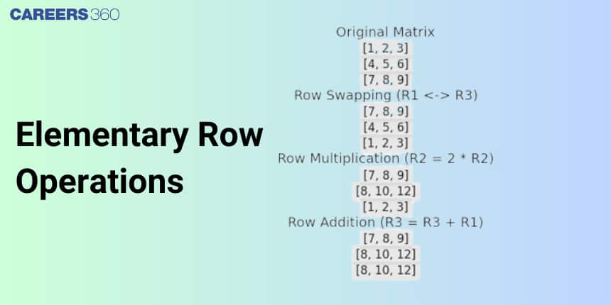
Elementary Row Operations

Row transformation: The following three types of operation (transformation) on the rows of a given matrix are known as elementary row operation (transformation).
i) Interchange of $\mathrm{i}^{\text {th }}$ row with $\mathrm{j}^{\text {th }}$ row, this operation is denoted by
$
R_{\mathrm{i}} \leftrightarrow R_{\mathrm{j}}
$

During this operation, all the elements of $\mathrm{i}^{\text {th }}$ row get replaced by all the elements of $\mathrm{j}^{\text {th }}$ row.
ii) The multiplication of $\mathrm{i}^{\text {th }}$ row by a constant $\mathrm{k}(\mathrm{k} \neq 0)$ is denoted by
$
\mathrm{R}_{\mathrm{i}} \leftrightarrow \mathrm{kR}_{\mathrm{i}}
$

During this operation, all the elements $\mathrm{i}^{\text {th }}$ row are replaced by multiplication of elements $\mathrm{i}^{\text {th }}$ row by the constant $\mathrm{k}$.
iii) Adding of $\mathrm{i}^{\text {th }}$ row elements with of $\mathrm{j}^{\text {th }}$ row multiplied by constant $k(k \neq 0)$ is denoted by
$
R_i \leftrightarrow R_i+k R_j
$

During this operation, $\mathrm{i}^{\text {th }}$ row elements are replaced by adding the previous value of the $\mathrm{i}^{\text {th }}$ row and elements of $j^{\text {th }}$ row multiplied by a constant ( $k$ ).

In the same way, three-column operations can also be defined.

Steps for finding the inverse of a matrix of order 2 by elementary row operations

Step i: Write $A=I_n A$
Step II: Perform a sequence of elementary row operations successively on A on the LHS and the prefactor $I_n$ on the RHS till we obtain the result $I_n=B A$
Step III: Write $A^{-1}=B$

Algorithm for finding the inverse of a singular 3 x 3 Matrix by Elementary Row Transformations

Introduce unity at the intersection of the first row and first column either by interchanging two rows or by adding a constant multiple of elements of some other row to the first row.
After introducing unity at (1,1) place introduce zeros at all other places in the first column.
Introduce unity at the intersection of the 2nd row and 2nd column with the help of the 2nd and 3rd row.
Introduce zeros at all other places in the second column except at the intersection of 2nd row and 2nd column.
Introduce unity at the intersection of 3rd row and third column.
Finally, introduce zeros at all other places in the third column except at the intersection of third row and third column.

JEE Main Highest Scoring Chapters & Topics

Focus on high-weightage topics with this eBook and prepare smarter. Gain accuracy, speed, and a better chance at scoring higher.

Download E-book

Elementary Column Transformation

In the Elementary column transformation, the matrices' columns are the only ones that are altered. The row remains unchanged. A predetermined set of guidelines is followed when performing these column operations to ensure that the transformed matrix is identical to the original matrix.

Solved Examples Based On Elementary Row Transformation

Example 1: Find the inverse of matrix A, if matrix A= $\left[\begin{array}{cc}a & b \\ c & \left(\frac{1+b c}{a}\right)\end{array}\right]$

Solution:

Use $\mathrm{A A^{-1}}=I$

$
\begin{aligned}
& {\left[\begin{array}{lc}
a & b \\
c & \left(\frac{1+b c}{a}\right)
\end{array}\right]=\left[\begin{array}{ll}
1 & 0 \\
0 & 1
\end{array}\right] \mathrm{A}} \\
& \mathrm{R}_1 \rightarrow \frac{1}{{a}} \mathrm{R}_1 \\
& {\left[\begin{array}{lc}
1 & \frac{b}{a} \\
c & \left(\frac{1+b c}{a}\right)
\end{array}\right]=\left[\begin{array}{ll}
\frac{1}{a} & 0 \\
0 & 1
\end{array}\right] \mathrm{A}} \\
& \mathrm{R}_2 \rightarrow \mathrm{R}_2-\mathrm{cR_{1 }} \\
& {\left[\begin{array}{ll}
1 & \frac{b}{q} \\
0 & \frac{1}{a}
\end{array}\right]=\left[\begin{array}{cc}
\frac{1}{a} & 0 \\
\frac{c}{a} & 1
\end{array}\right] \mathrm{A}} \\
& \mathrm{R}_2 \rightarrow \mathrm{aR}_2 \\
& {\left[\begin{array}{ll}
1 & \frac{b}{a} \\
0 & 1
\end{array}\right]=\left[\begin{array}{cc}
\frac{1}{a} & 0 \\
-c & a
\end{array}\right] \mathrm{A}} \\
& \mathrm{R}_2 \rightarrow \mathrm{R}_1-\frac{\mathrm{b}}{\mathrm{a}} \mathrm{R}_2 \\
& {\left[\begin{array}{ll}
1 & 0 \\
0 & 1
\end{array}\right]=\left[\begin{array}{cc}
\frac{1+b c}{a} & -b \\
-c & a
\end{array}\right] \mathrm{A}} \\
& \mathrm{A}^{-1}=\left[\begin{array}{cc}
\frac{1+b c}{a} & -b \\
-c & a
\end{array}\right]
\end{aligned}
$

Example 2: Find the inverse of a matrix $
\mathrm{A}=\left[\begin{array}{lll}
1 & 2 & 3 \\
0 & 1 & 2 \\
3 & 1 & 1
\end{array}\right]
$

Solution:
First write, $\mathrm{A}=\mathrm{IA}$
$
\Rightarrow\left[\begin{array}{lll}
1 & 2 & 3 \\
0 & 1 & 2 \\
3 & 1 & 1
\end{array}\right]=\left[\begin{array}{lll}
1 & 0 & 0 \\
0 & 1 & 0 \\
0 & 0 & 1
\end{array}\right] \mathrm{A}
$

Apply, $\mathrm{R}_3 \rightarrow \mathrm{R}_3-3 \mathrm{R}_1$
$
\Rightarrow\left[\begin{array}{ccc}
1 & 2 & 3 \\
0 & 1 & 2 \\
0 & -5 & -8
\end{array}\right]=\left[\begin{array}{ccc}
1 & 0 & 0 \\
0 & 1 & 0 \\
-3 & 0 & 1
\end{array}\right] \mathrm{A}
$

Apply, $\mathrm{R}_1 \rightarrow \mathrm{R}_1-2 \mathrm{R}_2$
$
\Rightarrow\left[\begin{array}{ccc}
1 & 0 & -1 \\
0 & 1 & 2 \\
0 & -5 & -8
\end{array}\right]=\left[\begin{array}{ccc}
1 & -2 & 0 \\
0 & 1 & 0 \\
-3 & 0 & 1
\end{array}\right] \mathrm{A}
$

Apply, $\mathrm{R}_3 \rightarrow \mathrm{R}_3+5 \mathrm{R}_2$
$
\Rightarrow\left[\begin{array}{ccc}
1 & 0 & -1 \\
0 & 1 & 2 \\
0 & 0 & 2
\end{array}\right]=\left[\begin{array}{ccc}
1 & -2 & 0 \\
0 & 1 & 0 \\
-3 & 5 & 1
\end{array}\right] \mathrm{A}
$

$
\begin{aligned}
& \text { Apply, } \mathrm{R}_3 \rightarrow \frac{1}{2} \mathrm{R}_3 \\
& \Rightarrow\left[\begin{array}{lll}
1 & 0 & -1 \\
0 & 1 & 2 \\
0 & 0 & 1
\end{array}\right]=\left[\begin{array}{ccc}
1 & -2 & 0 \\
0 & 1 & 0 \\
\frac{-3}{2} & \frac{5}{2} & \frac{1}{2}
\end{array}\right] \mathrm{A} \\
& \text { Apply, } \mathrm{R}_1 \rightarrow \mathrm{R}_1+\mathrm{R}_3 \\
& \Rightarrow\left[\begin{array}{lll}
1 & 0 & 0 \\
0 & 1 & 2 \\
0 & 0 & 1
\end{array}\right]=\left[\begin{array}{ccc}
-\frac{1}{2} & \frac{1}{2} & \frac{1}{2} \\
0 & 1 & 0 \\
\frac{-3}{2} & \frac{5}{2} & \frac{1}{2}
\end{array}\right] \mathrm{A} \\
& \text { Apply, } \mathrm{R}_2 \rightarrow \mathrm{R}_2-2 \mathrm{R}_3 \\
& \Rightarrow\left[\begin{array}{lll}
1 & 0 & 0 \\
0 & 1 & 0 \\
0 & 0 & 1
\end{array}\right]=\left[\begin{array}{ccc}
-\frac{1}{2} & \frac{1}{2} & \frac{1}{2} \\
3 & -4 & -1 \\
\frac{-3}{2} & \frac{5}{2} & \frac{1}{2}
\end{array}\right] \mathrm{A}
\end{aligned}
$

Hence, $
\mathrm{A}^{-1}=\left[\begin{array}{ccc}
-\frac{1}{2} & \frac{1}{2} & \frac{1}{2} \\
3 & -4 & -1 \\
\frac{-3}{2} & \frac{5}{2} & \frac{1}{2}
\end{array}\right]
$

Example 3 Find the inverse of the matrix $A=\left[\begin{array}{lll}1 & 2 & 0 \\ 3 & 2 & 5 \\ 1 & 2 & 3\end{array}\right]$
Solution
Use $A A^{-1}=I$
$
\begin{aligned}
& {\left[\begin{array}{lll}
1 & 2 & 0 \\
3 & 2 & 5 \\
1 & 2 & 3
\end{array}\right]=\left[\begin{array}{lll}
1 & 0 & 0 \\
0 & 1 & 0 \\
0 & 0 & 1
\end{array}\right] A} \\
& R_1 \leftrightarrow R_2 \\
& {\left[\begin{array}{lll}
3 & 2 & 5 \\
1 & 2 & 0 \\
1 & 2 & 3
\end{array}\right]=\left[\begin{array}{lll}
0 & 1 & 0 \\
1 & 0 & 0 \\
0 & 0 & 1
\end{array}\right] A}
\end{aligned}
$
$
\begin{aligned}
& R_2 \rightarrow R_2-\frac{1}{3} \cdot R_1 \\
& {\left[\begin{array}{ccc}
3 & 2 & 5 \\
0 & \frac{4}{3} & -\frac{5}{3} \\
1 & 2 & 3
\end{array}\right]=\left[\begin{array}{ccc}
0 & 1 & 0 \\
1 & -\frac{1}{3} & 0 \\
0 & 0 & 1
\end{array}\right] A} \\
& R_3 \rightarrow R_3-\frac{1}{3} \cdot R_1 \\
& {\left[\begin{array}{ccc}
3 & 2 & 5 \\
0 & \frac{4}{3} & -\frac{5}{3} \\
0 & \frac{4}{3} & \frac{4}{3}
\end{array}\right]=\left[\begin{array}{ccc}
0 & 1 & 0 \\
1 & -\frac{1}{3} & 0 \\
0 & -\frac{1}{3} & 1
\end{array}\right] A} \\
& R_3 \rightarrow R_3-1 \cdot R_2 \\
&
\end{aligned}
$

$\begin{aligned} & {\left[\begin{array}{ccc}3 & 2 & 5 \\ 0 & \frac{4}{3} & -\frac{5}{3} \\ 0 & 0 & 3\end{array}\right]=\left[\begin{array}{ccc}0 & 1 & 0 \\ 1 & -\frac{1}{3} & 0 \\ -1 & 0 & 1\end{array}\right] A} \\ & R_3 \rightarrow \frac{1}{3} \cdot R_3 \\ & {\left[\begin{array}{ccc}3 & 2 & 5 \\ 0 & \frac{4}{3} & -\frac{5}{3} \\ 0 & 0 & 1\end{array}\right]=\left[\begin{array}{ccc}0 & 1 & 0 \\ 1 & -\frac{1}{3} & 0 \\ -\frac{1}{3} & 0 & \frac{1}{3}\end{array}\right] A} \\ & R_2 \rightarrow R_2+\frac{5}{3} \cdot R_3 \\ & {\left[\begin{array}{lll}3 & 2 & 5 \\ 0 & \frac{4}{3} & 0 \\ 0 & 0 & 1\end{array}\right]=\left[\begin{array}{ccc}0 & 1 & 0 \\ \frac{4}{9} & -\frac{1}{3} & \frac{5}{9} \\ -\frac{1}{3} & 0 & \frac{1}{3}\end{array}\right] A} \\ & R_1 \rightarrow R_1-5 \cdot R_3 \\ & {\left[\begin{array}{lll}3 & 2 & 0 \\ 0 & \frac{4}{3} & 0 \\ 0 & 0 & 1\end{array}\right]=\left[\begin{array}{ccc}\frac{5}{3} & 1 & -\frac{5}{3} \\ \frac{4}{9} & -\frac{1}{3} & \frac{5}{9} \\ -\frac{1}{3} & 0 & \frac{1}{3}\end{array}\right] A} \\ & \end{aligned}$

$
\begin{aligned}
& R_2 \rightarrow \frac{3}{4} \cdot R_2 \\
& {\left[\begin{array}{lll}
3 & 2 & 0 \\
0 & 1 & 0 \\
0 & 0 & 1
\end{array}\right]=\left[\begin{array}{ccc}
\frac{5}{3} & 1 & -\frac{5}{3} \\
\frac{1}{3} & -\frac{1}{4} & \frac{5}{12} \\
-\frac{1}{3} & 0 & \frac{1}{3}
\end{array}\right] A} \\
& R_1 \rightarrow R_1-2 \cdot R_2 \\
& {\left[\begin{array}{lll}
3 & 0 & 0 \\
0 & 1 & 0 \\
0 & 0 & 1
\end{array}\right]=\left[\begin{array}{ccc}
1 & \frac{3}{2} & -\frac{5}{2} \\
\frac{1}{3} & -\frac{1}{4} & \frac{5}{12} \\
-\frac{1}{3} & 0 & \frac{1}{3}
\end{array}\right] A} \\
& R_1 \rightarrow \frac{1}{3} \cdot R_1 \\
& {\left[\begin{array}{lll}
1 & 0 & 0 \\
0 & 1 & 0 \\
0 & 0 & 1
\end{array}\right]=\left[\begin{array}{ccc}
\frac{1}{3} & \frac{1}{2} & -\frac{5}{6} \\
\frac{1}{3} & -\frac{1}{4} & \frac{5}{12} \\
-\frac{1}{3} & 0 & \frac{1}{3}
\end{array}\right] A} \\
& \text{Hence}, A^{-1}=\left[\begin{array}{ccc}
\frac{1}{3} & \frac{1}{2} & -\frac{5}{6} \\
\frac{1}{3} & -\frac{1}{4} & \frac{5}{12} \\
-\frac{1}{3} & 0 & \frac{1}{3}
\end{array}\right] \\
&
\end{aligned}
$

Example 4: Find the inverse matrix of $
A=\left[\begin{array}{rrr}
1 & 1 & 2 \\
2 & 3 & 5 \\
-1 & 0 & 2
\end{array}\right]
$

Solution:
Use $A A^{-1}=I$
$
\left[\begin{array}{rrr}
1 & 1 & 2 \\
2 & 3 & 5 \\
-1 & 0 & 2
\end{array}\right]=\left[\begin{array}{lll}
1 & 0 & 0 \\
0 & 1 & 0 \\
0 & 0 & 1
\end{array}\right] A
$

Swap matrix rows: $R_1 \leftrightarrow R_2$
$
\begin{aligned}
& {\left[\begin{array}{ccc}
2 & 3 & 5 \\
1 & 1 & 2 \\
-1 & 0 & 2
\end{array}\right]=\left[\begin{array}{lll}
0 & 1 & 0 \\
1 & 0 & 0 \\
0 & 0 & 1
\end{array}\right] A} \\
& R_2 \leftarrow R_2-\frac{1}{2} \cdot R_1 \\
& {\left[\begin{array}{ccc}
2 & 3 & 5 \\
0 & -\frac{1}{2} & -\frac{1}{2} \\
-1 & 0 & 2
\end{array}\right]=\left[\begin{array}{ccc}
0 & 1 & 0 \\
1 & -\frac{1}{2} & 0 \\
0 & 0 & 1
\end{array}\right] A}
\end{aligned}
$

$
\begin{gathered}
R_3 \leftarrow R_3+\frac{1}{2} \cdot R_1 \\
{\left[\begin{array}{ccc}
2 & 3 & 5 \\
0 & -\frac{1}{2} & -\frac{1}{2} \\
0 & \frac{3}{2} & \frac{9}{2}
\end{array}\right]=\left[\begin{array}{ccc}
0 & 1 & 0 \\
1 & -\frac{1}{2} & 0 \\
0 & \frac{1}{2} & 1
\end{array}\right]}
\end{gathered}
$

Swap matrix rows : $R_2 \leftrightarrow R_3$
$
\begin{aligned}
& {\left[\begin{array}{ccc}
2 & 3 & 5 \\
0 & \frac{3}{2} & \frac{9}{2} \\
0 & -\frac{1}{2} & -\frac{1}{2}
\end{array}\right]=\left[\begin{array}{ccc}
0 & 1 & 0 \\
0 & \frac{1}{2} & 1 \\
1 & -\frac{1}{2} & 0
\end{array}\right] A} \\
& R_3 \rightarrow R_3+\frac{1}{3} \cdot R_2 \\
& {\left[\begin{array}{lll}
2 & 3 & 5 \\
0 & \frac{3}{2} & \frac{9}{2} \\
0 & 0 & 1
\end{array}\right]=\left[\begin{array}{ccc}
0 & 1 & 0 \\
0 & \frac{1}{2} & 1 \\
1 & -\frac{1}{3} & \frac{1}{3}
\end{array}\right] A} \\
& R_2 \rightarrow R_2-\frac{9}{2} \cdot R_3 \\
& {\left[\begin{array}{lll}
2 & 3 & 5 \\
0 & \frac{3}{2} & 0 \\
0 & 0 & 1
\end{array}\right]=\left[\begin{array}{ccc}
0 & 1 & 0 \\
-\frac{9}{2} & 2 & -\frac{1}{2} \\
1 & -\frac{1}{3} & \frac{1}{3}
\end{array}\right] A} \\
& R_1 \rightarrow R_1-5 \cdot R_3 \\
&
\end{aligned}
$

$\begin{aligned} & {\left[\begin{array}{lll}2 & 3 & 0 \\ 0 & \frac{3}{2} & 0 \\ 0 & 0 & 1\end{array}\right]=\left[\begin{array}{ccc}-5 & \frac{8}{3} & -\frac{5}{3} \\ -\frac{9}{2} & 2 & -\frac{1}{2} \\ 1 & -\frac{1}{3} & \frac{1}{3}\end{array}\right] A} \\ & R_2 \rightarrow \frac{2}{3} \cdot R_2 \\ & {\left[\begin{array}{lll}2 & 3 & 0 \\ 0 & 1 & 0 \\ 0 & 0 & 1\end{array}\right]=\left[\begin{array}{ccc}-5 & \frac{8}{3} & -\frac{5}{3} \\ -3 & \frac{4}{3} & -\frac{1}{3} \\ 1 & -\frac{1}{3} & \frac{1}{3}\end{array}\right] A} \\ & R_1 \rightarrow R_1-3 \cdot R_2 \\ & {\left[\begin{array}{lll}2 & 0 & 0 \\ 0 & 1 & 0 \\ 0 & 0 & 1\end{array}\right]=\left[\begin{array}{ccc}4 & -\frac{4}{3} & -\frac{2}{3} \\ -3 & \frac{4}{3} & -\frac{1}{3} \\ 1 & -\frac{1}{3} & \frac{1}{3}\end{array}\right] A} \\ & \end{aligned}$

$
\begin{aligned}
& \qquad R_1 \rightarrow \frac{1}{2} \cdot R_1 \\
& {\left[\begin{array}{lll}
1 & 0 & 0 \\
0 & 1 & 0 \\
0 & 0 & 1
\end{array}\right]=\left[\begin{array}{ccc}
2 & -\frac{2}{3} & -\frac{1}{3} \\
-3 & \frac{4}{3} & -\frac{1}{3} \\
1 & -\frac{1}{3} & \frac{1}{3}
\end{array}\right] A} \\
\end{aligned}
$

Hence, $
A^{-1}=\left[\begin{array}{ccc}
2 & -\frac{2}{3} & -\frac{1}{3} \\
-3 & \frac{4}{3} & -\frac{1}{3} \\
1 & -\frac{1}{3} & \frac{1}{3}
\end{array}\right]
$

Frequently Asked Questions (FAQs)

Q: How do elementary row operations relate to the concept of matrix similarity?

Elementary row operations do not preserve matrix similarity. Similar matrices share properties like eigenvalues and determinants, but row operations can change these. This distinction is important in understanding the limitations of row operations in certain matrix analyses, particularly those involving eigenvalue problems.

Q: What is the significance of partial pivoting in row reduction algorithms?

Partial pivoting involves selecting the largest absolute value in a column as the pivot during row reduction. This technique is crucial in numerical computations to minimize rounding errors and improve the stability of the algorithm, especially for matrices with widely varying element magnitudes.

Q: How do you use elementary row operations to find a basis for the row space of a matrix?

To find a basis for the row space, use elementary row operations to reduce the matrix to row echelon form. The non-zero rows of this reduced matrix form a basis for the row space. This works because row operations preserve the row space while simplifying the matrix structure.

Q: What is the role of elementary row operations in solving matrix equations?

In solving matrix equations like AX = B, elementary row operations are applied to the augmented matrix [A|B]. By reducing this to row echelon or reduced row echelon form, we can solve for X. This method extends the concept of solving linear systems to matrix-valued unknowns.

Q: How do elementary row operations relate to the concept of matrix equivalence?

Two matrices are row equivalent if one can be obtained from the other through a sequence of elementary row operations. This equivalence is crucial because row equivalent matrices represent the same linear system and share many important properties, such as rank and solution sets.

Q: What is the connection between elementary row operations and Gaussian elimination?

Gaussian elimination is essentially a systematic application of elementary row operations. It uses these operations in a specific order to transform a matrix into row echelon form, which is crucial for solving systems of linear equations and analyzing matrix properties.

Q: How do elementary row operations affect the nullity of a matrix?

Elementary row operations do not change the nullity of a matrix. The nullity, which is the dimension of the null space, remains constant because row operations preserve the fundamental solution space of the homogeneous system Ax = 0.

Q: What is the significance of a zero row in row reduction?

A zero row obtained through row reduction indicates linear dependence among the original equations in a system. In terms of matrix rank, each zero row reduces the rank by one. In solving systems, zero rows often correspond to redundant or trivially satisfied equations.

Q: What is the role of elementary row operations in computing matrix determinants?

While elementary row operations can change the determinant value, they do so in predictable ways. This property is often used in determinant calculations: reduce the matrix to triangular form using row operations, keeping track of how these operations affect the determinant, then compute the product of diagonal elements.

Q: What is the significance of back-substitution in row reduction methods?

Back-substitution is the final step in solving systems using row reduction. After obtaining row echelon form, you work backwards from the bottom row, substituting known values to find the remaining unknowns. This step is crucial for obtaining explicit solutions from the reduced matrix.

Articles

Tamil Nadu BSc Nursing Admission 2025: Counselling (Started), Seat Matrix, Merit List

Sep 12, 2025

DU LLB Fee Structure 2026 - Check Complete Details

Sep 11, 2025

Top 5 Career Options after B.Arch - Eligibility, Salary Trends

Sep 11, 2025

Top 6 Career Options after BAF - Eligibility, Salary

Sep 06, 2025