Random Variables and its Probability Distributions

Random Variable and probability distribution are important concepts of probability. If the value of a random variable together with the corresponding probabilities are given then this description is called a probability distribution of the random variable. These concepts help the analyst analyze the decisions in various fields like science, commerce, etc.

Random Variable

A random variable is a real-valued function whose domain is the sample space of a random experiment. It is a numerical description of the outcome of a statistical experiment.
A random variable is usually denoted by $X$.
For example, consider the experiment of tossing a coin two times in succession. The sample space of the experiment is $S=\{H H, H T, T H, T T\}$.
If $X$ is the number of tails obtained, then $X$ is a random variable and for each outcome, its value is given as

$
X(T T)=2, X(H T)=1, X(T H)=1, X(H H)=0
$

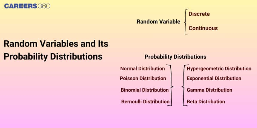
Types Of Random Variables:
1. Discrete Random Variable: Discrete random variable can take finite unique variables.
2. Continuous Random Variable: A continuous random variable can take infinite no. of values in a range.

Probability Distribution of a Random Variable
The probability distribution for a random variable describes how the probabilities are distributed over the values of the random variable.
The probability distribution of a random variable $X$ is the system of numbers

$
\begin{array}{rlllllll}
X & : & x_1 & x_2 & x_3 & \ldots & \ldots & x_n \\
P(X) & : & p_1 & p_2 & p_3 & \ldots & \ldots & p_n \\
& p_i \neq 0, & \sum_{i=1}^n p_i=1, & i=1,2,3, \ldots n
\end{array}
$

The real numbers $\underline{\underline{x_1},}, x_2, \ldots, x_n$ are the possible values of the random variable $X$ and $p_i(i=1,2, \ldots, n)$ is the probability of the random variable $X$ taking the value $x i$ i.e., $P\left(X=x_i\right)=p_i$
Types Of Probability Distribution:
1. Binomial distribution
2. Normal Distribution
3. Cumulative distribution frequency

The mean of a Random Variable
Let X be a random variable whose possible values $\underline{\mathrm{x}_1}, \underline{\mathrm{x}_2}, \ldots, \mathrm{x}_{\mathrm{n}}$ occur with probabilities $\underline{\underline{p_1}}, \underline{\mathrm{p}_2}, \underline{\mathrm{p}_3}, \ldots, \mathrm{p}_{\mathrm{n}}$, respectively. The mean of X , denoted by $\mu$, is the number $\sum_{i=1}^n x_i p_i$ i.e. the mean of X is the weighted average of the possible values of $X$, each value being weighted by its probability with which it occurs.
।
The mean of a random variable X is also called the expectation of X , denoted by $\mathrm{E}(\mathrm{X})$.

$
\begin{array}{|c|c|c|}
\hline \text { Random variable }\left(\mathrm{x}_{\mathrm{i}}\right) & \text { Probability }\left(\mathrm{p}_{\mathrm{i}}\right) & \mathrm{p}_{\mathrm{i}} \mathrm{x}_{\mathrm{i}} \\
\hline \mathrm{x}_1 & \mathrm{p}_1 & \mathrm{p}_1 \mathrm{x}_1 \\
\hline \mathrm{x}_2 & \mathrm{p}_2 & \mathrm{p}_2 \mathrm{x}_2 \\
\hline \mathrm{x}_3 & \mathrm{p}_3 & \mathrm{p}_3 \mathrm{x}_3 \\
\hline \ldots & \ldots & \ldots \\
\hline \ldots & \ldots & \ldots \\
\hline \mathrm{x}_{\mathrm{n}} & \mathrm{p}_n & \mathrm{p}_n \mathrm{x}_n \\
\hline
\end{array}$

Thus,

$
\operatorname{mean}(\mu)=\frac{\sum_{i=1}^n p_i x_i}{\sum_{i=1}^n p_i}=\sum_{i=1}^n x_i p_i \quad\left(\because \sum_{i=1}^n p_i=1\right)
$

Variance of a random variable
Let $X$ be a random variable whose possible values $x_1, x_2, \ldots, x_n$ occur with probabilities $p\left(x_1\right), p\left(x_2\right), \ldots, p\left(x_n\right)$ respectively.
Let $\mu=\mathrm{E}(\mathrm{X})$ be the mean of X . The variance of X , denoted by $\operatorname{Var}(\mathrm{X})$ or $\sigma_x^2$ is defined as

$
\sigma_x^2=\operatorname{Var}(\mathrm{X})=\sum_{i=1}^n\left(x_i-\mu\right)^2 p\left(x_i\right)
$

And the non-negative number

$
\sigma_x=\sqrt{\operatorname{Var}(\mathrm{X})}=\sqrt{\sum_{i=1}^n\left(x_i-\mu\right)^2 p\left(x_i\right)}
$

is called the standard deviation of the random variable $\mathbf{X}$. Mastery of these concepts can help in solving gaining deeper insights and contributing meaningfully to real-life problems.

Solved Examples Based on Random Variable and Probability Distribution:

Example 1: Each of the two persons $A$ and $B$ toss a fair coin simultaneously 50 times. The probability that both of them will not get head at the same toss is
1) $\left(\frac{3}{4}\right)^{50}$
2) $\left(\frac{2}{7}\right)^{50}$
3) $\left(\frac{1}{8}\right)^{50}$
4) $\left(\frac{7}{8}\right)^{50}$

Solution
Probability of Distribution of the Random Variable -
If the value of a random variable together with the corresponding probabilities are given then this description is called a probability distribution of the random variable.
At any trial, four cases arise
(i) both $A$ and $B$ get head
(ii) $A$ gets head, $B$ gets tail
(iii) $A$ gets tail, $B$ gets head
(iv) both get tail

$P$ (they do not get head simultaneously on a particular trail $=\frac{3}{4}$
$P($ they do not get heads simultaneously in 50 trials $)=\left(\frac{3}{4}\right)^{50}$

Hence, the answer is option 1.

Example 2: Two numbers are selected at random (without replacement) from the first six positive integers. If $X$ denotes the smaller of the two numbers, then the expectation of $X$ is :
1) $\frac{5}{3}$
2) $\frac{14}{3}$
3) $\frac{13}{3}$
4) $\frac{7}{3}$

Solution
The two positive integers can be selected from the first six positive integers without replacement in $6 \times 5=30$ ways.
$X$ represents the larger of the two numbers obtained. Therefore, $X$ can take the value of $2,3,4,5$, or 6 .
For $X=2$, the possible observations are $(1,2)$ and $(2,1)$.

$
\therefore P(X=2)=\frac{2}{30}=\frac{1}{15}
$
For $X=3$, the possible observations are $(1,3),(2,3),(3,1)$, and $(3,2)$.

$
\therefore P(X=3)=\frac{4}{30}=\frac{2}{15}
$

For $X=4$, the possible observations are $(1,4),(2,4),(3,4),(4,3),(4,2)$, and $(4,1)$.

$
\therefore P(X=4)=\frac{6}{30}=\frac{1}{5}
$

For $\mathrm{X}=5$, the possible observations are $(1,5),(2,5),(3,5),(4,5),(5,4),(5,3),(5,2)$, and $(5,1)$.

$
\therefore P(X=5)=\frac{8}{30}=\frac{4}{15}
$

For $X=6$, the possible observations are $(1,6),(2,6),(3,6),(4,6),(5,6),(6,4),(6,3),(6,2)$, and $(6,1)$.

$
\therefore P(X=6)=\frac{10}{30}=\frac{1}{3}
$
Therefore, the required probability distribution is as follows.

$
\begin{aligned}
& \text { Then, } E(X)=\sum X_i P\left(X_i\right) \\
& =2 \cdot \frac{1}{15}+3 \cdot \frac{2}{15}+4 \cdot \frac{1}{5}+5 \cdot \frac{4}{15}+6 \cdot \frac{1}{3} \\
& =\frac{2}{15}+\frac{2}{5}+\frac{4}{5}+\frac{4}{3}+2 \\
& =\frac{70}{15} \\
& =\frac{14}{3}
\end{aligned}
$
Hence, the answer is the option 2.

Example 3: A random variable $X$ has the following probability distribution:

$
\begin{array}{rccccc}
X: & 1 & 2 & 3 & 4 & 5 \\
P(X): & K^2 & 2 K & K & 2 K & 5 K^2
\end{array}
$
Then $P(X>2)$ is equal to:
1) $\frac{7}{12}$
2) $\frac{23}{36}$
3) $\frac{1}{36}$
4) $\frac{1}{6}$

Solution

$
\begin{aligned}
& \sum P_i=1 \Rightarrow 6 k^2+5 k=1 \\
& \Rightarrow 6 k^2+5 k-1=0 \\
& \Rightarrow k=\frac{1}{6}, k=-1 \text { (invalid) } \\
& \text { Now, } P(X>2)=P(3)+P(4)+P(5)=k+2 k+5 k^2 \\
& =\frac{1}{6}+\frac{2}{6}+\frac{5}{36}=\frac{6+12+5}{36}=\frac{23}{36}
\end{aligned}
$
Hence, the answer is the option 2.

Example 4: A random variable $X$ has the following probability distribution:

The value of $P(1<X<4 \mid X \leq 2)$ is equal to:
1) $\frac{4}{7}$
2) $\frac{2}{3}$
3) $\frac{3}{7}$
4) $\frac{4}{5}$

Solution

$
\begin{aligned}
& \mathrm{k}+2 \mathrm{k}+4 \mathrm{k}+6 \mathrm{k}+8 \mathrm{k}=1 \\
& \mathrm{k}=\frac{1}{21}=\frac{\mathrm{p}(\mathrm{x}=2)}{\mathrm{p}(\mathrm{x} \leq 2)} \\
& \mathrm{P}(1<\mathrm{x}<4 / \mathrm{x} \leq 2)= \frac{4 \mathrm{k}}{\mathrm{k}+2 \mathrm{k}+4 \mathrm{k}} \\
&=\frac{4}{7}
\end{aligned}
$
Hence, the answer is the option (1).

Example 5: A six-faced die is biased such that $3 \times \mathrm{P}$ (a prime number) $=6 \times \mathrm{P}$ (a composite number) $=2 \times \mathrm{P}(1)$. Let X be a random variable that counts the number of times one gets a perfect square on some throws of this die. If the die is thrown twice, then the mean of X is
1) $\frac{3}{11}$
2) $\frac{5}{11}$
3) $\frac{7}{11}$
4) $\frac{8}{11}$

Solution
Let $\mathrm{P}(1)=\mathrm{k}$
$\therefore \quad \mathrm{P}(2)=\mathrm{P}(3)=\mathrm{P}(5)=\frac{2 \mathrm{k}}{3}$ and $\mathrm{P}(4)=\mathrm{P}(6)=\frac{\mathrm{k}}{3}$
As Sum=1

$
\begin{aligned}
& \mathrm{k}+(2 \mathrm{k})+\frac{2 \mathrm{k}}{3}=1 \\
& \Rightarrow \mathrm{k}=\frac{3}{11}
\end{aligned}
$
Now $\mathrm{n}=2$
and $\mathrm{P}=\mathrm{P}(1)+\mathrm{P}(4)=\mathrm{k}+\frac{\mathrm{k}}{3}=\frac{4 \mathrm{k}}{3}$ $=\frac{4}{11}$
$\therefore$ Mean $=\mathrm{np}=2 \times \frac{4}{11}=\frac{8}{11}$
$\therefore$ Option(D)
Hence, the answer is the option 4.

Summary
A random variable is a real-valued function whose domain is the sample space of a random experiment. It is a numerical description of the outcome of a statistical experiment. These methods are widely used in real-life applications providing insights and solutions to complex problems. Mastery of these concepts can help in solving gaining deeper insights and contributing meaningfully to real-life problems.